
This topic explains the method to perform binary classification using logistic regression from scratch using python.
What is Logistic Regression? Why it is used for classification?
Logistic regression is a statistical model used to analyze the dependent variable is dichotomous (binary) using logistic function. As the logistic or sigmoid function used to predict the probabilities between 0 and 1, the logistic regression is mainly used for classification.
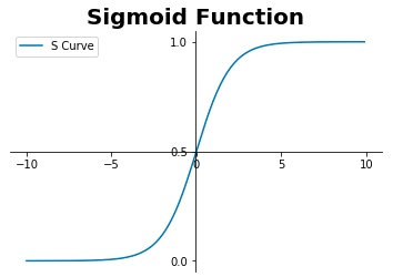
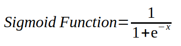
What is Logistic or Sigmoid Function?
As per Wikepedia, “A sigmoid function is a mathematical function having a characteristic “S”-shaped curve or sigmoid curve.” The output of sigmoid function results from 0 to 1 in a continous scale.
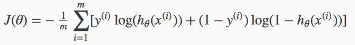
Why we need to use cross entropy cost function rather than mean squared error for logistic regression?
Cross-entropy cost function measures the performance of a classification model whose output is a probability value between 0 and 1. It is also called log loss.
In linear regression, we need to minimize the mean squared error using any optimization algorithm because the cost function is a convex function. It has only one local or global minima.
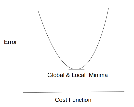
In logistic regression, if we use mean square error cost function with logistic function, it provides non-convex outcome which results in many local minima.
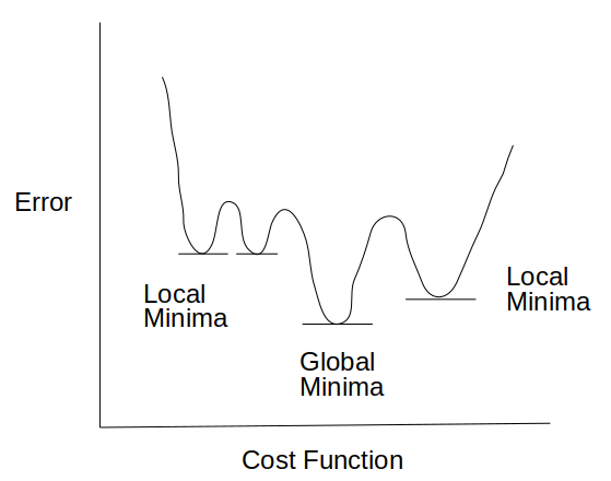
cross entropy cost function with logistic function gives convex curve with one local/global minima.
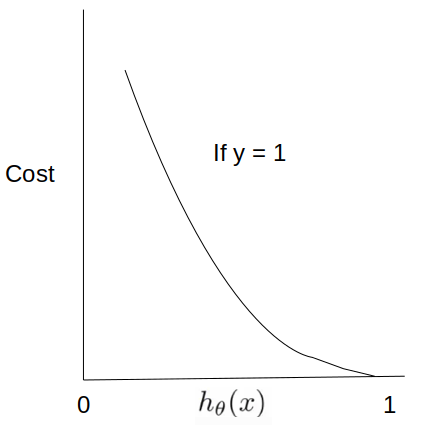
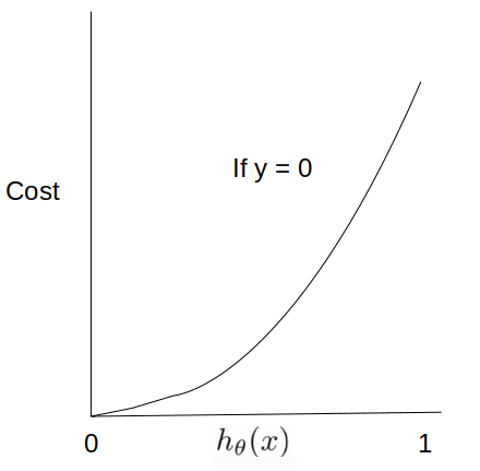
As per the below figures, cost entropy function can be explained as follows:
1) if actual y = 1, the cost or loss reduces as the model predicts the exact outcome.
2) if actual y = 0, the cost pr loss increases as the model predicts the wrong outcome.
So If we join both the below curves, it is a convex with one global minima to predict the correct outcome (0 or 1)
How to determine the number of model parameters?
1) The number of model parameters(Theta) depends upon the number of independent variables.
2) For example, if we need to perform claasification using linear decision boundary and 2 independent variables available, the number of model parameters is 3.
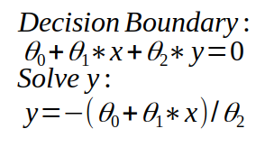
How to determine the decision boundary for logistic regression?
Decision boundary is calculated as follows:
Below is an example python code for binary classification using Logistic Regression
import numpy as np
import pandas as pd
from sklearn.metrics import confusion_matrix
import matplotlib.pyplot as plt
Function to create random data for classification
def random():
    X1 = []
    X2 = []
    y = []

    np.random.seed(1)
    for i in range(0,20):
        X1.append(i)
        X2.append(np.random.randint(100))
        y.append(0)

    for i in range(20,50):
        X1.append(i)
        X2.append(np.random.randint(80,300))
        y.append(1)

    return X1,X2,y
def standardize(data):
    data -= np.mean(data)
    data /= np.std(data)
    return data
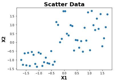
def plot(X):
    plt.scatter(X[:,0],X[:,1])
    plt.xlabel('X1',fontweight="bold",fontsize = 15)
    plt.ylabel('X2',fontweight="bold",fontsize = 15)
    plt.title("Scatter Data",fontweight="bold",fontsize = 20)
    plt.show()
Sigmoid Function used for Binary Classification
def sigmoid(X,theta):
    z = np.dot(X,theta.T)
    return 1.0/(1+np.exp(-z))
Cross-entropy cost function measures the performance of a classification model whose output is a probability value between 0 and 1. It is also called log loss.
def cost_function(h,y):
    loss = ((-y * np.log(h))-((1-y)* np.log(1-h))).mean()
    return loss
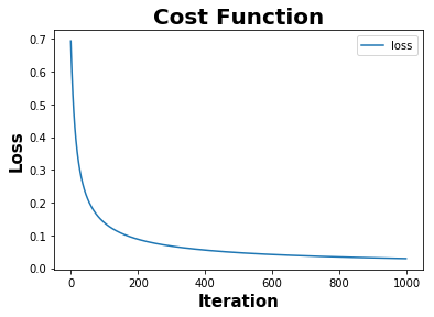
Gradient descent algorithm used to optimize the model parameters(theta) by minimizing the log loss.
def gradient_descent(X,h,y):
    return np.dot(X.T,(h-y))/y.shape[0]
def update_loss(theta,learning_rate,gradient):
    return theta-(learning_rate*gradient)
def predict(X,theta):
    threshold = 0.5
    outcome = []
    result = sigmoid(X,theta)
    for i in range(X.shape[0]):
        if result[i] <= threshold:
            outcome.append(0)
        else:
            outcome.append(1)
    return outcome
def plot_cost_function(cost):
    plt.plot(cost,label="loss")
    plt.xlabel('Iteration',fontweight="bold",fontsize = 15)
    plt.ylabel('Loss',fontweight="bold",fontsize = 15)
    plt.title("Cost Function",fontweight="bold",fontsize = 20)
    plt.legend()
    plt.show()
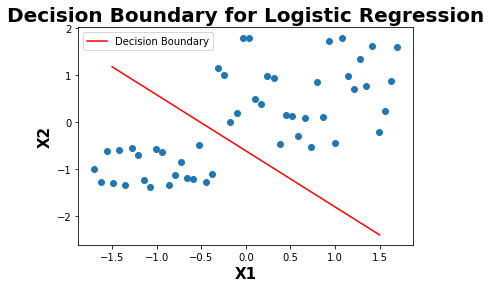
def plot_predict_classification(X,theta):
    plt.scatter(X[:,1],X[:,2])
    plt.xlabel('X1',fontweight="bold",fontsize = 15)
    plt.ylabel('X2',fontweight="bold",fontsize = 15)
    x = np.linspace(-1.5, 1.5, 50)
    y = -(theta[0] + theta[1]*x)/theta[2]
    plt.plot(x,y,color="red",label="Decision Boundary")
    plt.title("Decision Boundary for Logistic Regression",fontweight="bold",fontsize = 20)
    plt.legend()
    plt.show()
if __name__ == "__main__":
X1,X2,y = random()
X1 = standardize(X1)
X2 = standardize(X2)
X = np.array(list(zip(X1,X2)))
y = np.array(y)
plot(X)
# Feature Length
m = X.shape[0]
# No. of Features
n = X.shape
# No. of Classes
k = len(np.unique(y))
# Initialize intercept with ones
intercept = np.ones((X.shape[0],1))
X = np.concatenate((intercept,X),axis= 1)
# Initialize theta with zeros
theta = np.zeros(X.shape[1])
num_iter = 1000
cost = []
for i in range(num_iter):
h = sigmoid(X,theta)
cost.append(cost_function(h,y))
gradient = gradient_descent(X,h,y)
theta = update_loss(theta,0.1,gradient)
outcome = predict(X,theta)
plot_cost_function(cost)
print("theta_0 : {} , theta_1 : {}, theta_2 : {}".format(theta[0],theta[1],theta[2]))
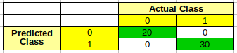
metric = confusion_matrix(y,outcome)
print(metric)
plot_predict_classification(X,theta)
Calculated Model Parameters:
theta_0 : 1.731104110180229 , theta_1 : 3.384426535937368, theta_2 : 2.841095441821299
Confusion Matrix:
[[20  0]
 [ 0 30]]
References :
- https://en.wikipedia.org/wiki/Logistic_regression
- https://en.wikipedia.org/wiki/Sigmoid_function
- https://en.wikipedia.org/wiki/Logistic_function
Comments