Cost Function Optimization using Gradient Descent Algorithm − Blog by dchandra

This topic explains the cost function optimization using Gradient Descent Algorithm.

What is Cost Function?

First of all, Cost Function can be also called as Loss Function. It typically represents the error of the trained model performance.

The objective of a cost function can be different for different machine learning algorithms.

minimize mean squared error (Linear Regression)
maximize the reward function (reinforcement learning)
minimize Gini index/maximize information gain (Decision tree classification)
minimize cross entropy (Logistic Regression)

What is Gradient and how it differs from derivative?

As per Wikepedia, “The gradient is a multi-variable generalization of the derivative. While a derivative can be defined on functions of a single variable, for functions of several variables, the gradient takes its place. The gradient is a vector-valued function, as opposed to a derivative, which is scalar-valued Like the derivative, the gradient represents the slope of the tangent of the graph of the function.”

What is the relationship between cost function and gradient descent?

Any cost function can be minimized or maximized using gradients. The gradient vector helps to find out the direction to optimize and its magnitude represents the slope of the function in that direction.

Below is an example to optimize the linear regression cost function using gradient descent algorithm

# Import libraries for basic python operation

import numpy as np
import matplotlib.pyplot as plt
%matplotlib inline

Function to generate random numbers

def random():
    np.random.seed(1) # generate same numbers
    X = np.arange(50)
    delta = np.random.uniform(0,15,size=(50,))
    y = .4 * X + 3 + delta
    return X,y

Data Normalization

def normalize(data):
    data -= np.min(data)
    data /= np.ptp(data)
    return data

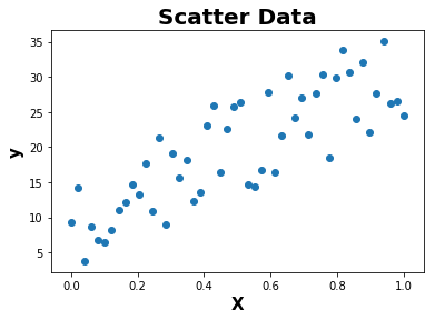
def plot(X,y):
    plt.scatter(X,y)
    plt.xlabel('X',fontweight="bold",fontsize = 15)
    plt.ylabel('y',fontweight="bold",fontsize = 15)
    plt.title('Scatter Data',fontweight="bold",fontsize = 20)
    plt.show()

Gradient Descent Algorithm

def gradient_descent(X,y):
    m_updated = 0
    b_updated = 0
    mse = []
    iterations = 500
    learning_rate = 0.01
    n = len(X)

    for i in range(iterations):
        y_pred = (X * m_updated) + b_updated

        error = y_pred - y

        mse.append(np.mean(np.square(error)))

        m_grad = 2/n * np.matmul(np.transpose(X),error)
        b_grad = 2 * np.mean(error)

        m_updated -= learning_rate * m_grad
        b_updated -= learning_rate * b_grad


    return [m_updated,b_updated,mse]

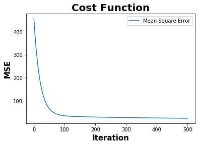
The objective of the cost function is to minimize the mean squared error.

def plot_cost_function(mse):
    plt.plot(mse,label="Mean Square Error")
    plt.xlabel('Iteration', fontweight="bold", fontsize = 15)
    plt.ylabel('MSE', fontweight="bold", fontsize = 15)
    plt.title('Cost Function',fontweight="bold",fontsize = 20)
    plt.legend()
    plt.show()   

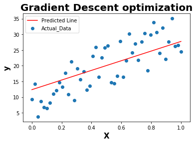
def plot_line(X,y,y_pred):
    plt.scatter(X,y,label="Actual_Data")
    plt.plot(X,y_pred,c='r',label = "Predicted Line")
    plt.xlabel('X', fontweight="bold", fontsize = 15)
    plt.ylabel('y', fontweight="bold", fontsize = 15)
    plt.title('Gradient Descent optimization',fontweight="bold",fontsize = 20)
    plt.legend()
    plt.show()  

if __name__ == "__main__":

    X,y = random()

    X = np.array(X).astype(np.float32)
    y = np.array(y).astype(np.float32)
    X = X.reshape(-1,1)
    y = y.reshape(-1,1)

    # Normalize the features
    X = normalize(X)

    plot(X,y)

    m,b,mse = gradient_descent(X,y)

    plot_cost_function(mse)

    y_pred = m * X + b

    plot_line(X,y,y_pred)