Linear Regression using sklearn

This topic explains the basics of regression with a simple linear regression program and validating the output using the metrics.

Regression

Regression analysis is a form of predictive modelling technique which investigates the relationship between a dependent (target) and independent variable (s) (predictor). This technique is used for forecasting, time series modelling and finding the causal effect relationship between the variables.

The two main benifits of regression analysis is as follows:

1. It indicates the significant relationships between dependent variable and independent variable.
2. It indicates the strength of impact of multiple independent variables on a dependent variable.

Regression analysis is an important tool for modelling and analyzing data. Here, we fit a curve / line to the data points, in such a manner that the differences between the distances of data points from the curve or line is minimized.

Regression metrics

Before understanding the metrics, we need to understand the most important concept in regression.

1. Overfitting
Overfitting occurs when a statistical model or machine learning algorithm captures the noise of the data. Intuitively, overfitting occurs when the model or the algorithm fits the data too well. Specifically, overfitting occurs if the model or algorithm shows low bias but high variance. Overfitting is often a result of an excessively complicated model, and it can be prevented by fitting multiple models and using validation or cross-validation to compare their predictive accuracies on test data.
2. Underfitting
Underfitting occurs when a statistical model or machine learning algorithm cannot capture the underlying trend of the data. Intuitively, underfitting occurs when the model or the algorithm does not fit the data well enough. Specifically, underfitting occurs if the model or algorithm shows low variance but high bias. Underfitting is often a result of an excessively simple model.

Both overfitting and underfitting lead to poor predictions on new data sets.

The three important metrics for regression :

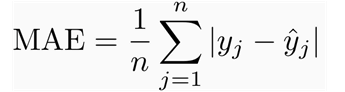
1. Mean absolute error This measure gives an idea of the magnitude of the error, but no direction.It’s the average over the test sample of the absolute differences between prediction and actual observation where all individual differences have equal weight.

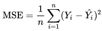
2. Mean squared error In statistics, the mean squared error (MSE) or mean squared deviation (MSD) of an estimator (of a procedure for estimating an unobserved quantity) measures the average of the squares of the errors—that is, the average squared difference between the estimated values and what is estimated.

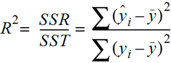
3. Coefficient of determination This measure provides an indication of the goodness of fit of a set of predictions to the actual values. It is also referered as R².

Below code is a simple example of a linear regression.

import numpy as np
import random
import pandas as pd

import matplotlib.pyplot as plt
%matplotlib inline

from sklearn import model_selection, cross_validation
from sklearn.linear_model import LinearRegression
from sklearn.preprocessing import PolynomialFeatures
from sklearn.metrics import regression
from sklearn import metrics

def read_data():
    data = pd.read_csv('data-scatter.csv')
    return data    

Download the data-scatter.csv

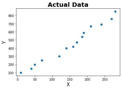
def plot(data):
    X = data['X']
    y = data['y']
    plt.scatter(X,y)
    plt.xlabel('X', fontsize = 15)
    plt.ylabel('Y', fontsize = 15)
    plt.title('Actual Data',fontweight="bold",fontsize = 20)
    plt.show()

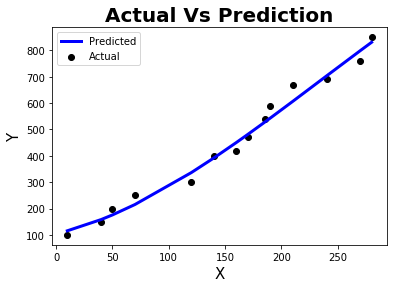
def plot_line(X,y,y_pred_line):
    plt.scatter(X, y,  color='black', label = 'Actual')
    plt.plot(X, y_pred_line, color='blue', linewidth=3, label = 'Predicted')
    plt.xlabel('X', fontsize = 15)
    plt.ylabel('Y', fontsize = 15)
    plt.title('Actual Vs Prediction',fontweight="bold",fontsize = 20)
    plt.legend()
    plt.show()

def polynomial(data):
    X = data['X']
    y = data['y']
    X = X.values.reshape(-1,1)
    poly = PolynomialFeatures(degree=3)
    X = poly.fit_transform(X)
    return X,y

def split_data(X,y,seed):
    kf = model_selection.KFold(n_splits = 3, shuffle = True, random_state = seed)
    for train_index, test_index in kf.split(X):
        X_train, X_test = X[train_index], X[test_index]
        y_train, y_test = y[train_index], y[test_index]
    return X_train,X_test,y_train,y_test

def model(X_train,X_test,y_train,y_test):
    model = LinearRegression(normalize=True)
    model.fit(X_train,y_train)
    y_pred = model.predict(X_test)
    y_pred_line = model.predict(X)
    return y_pred, y_pred_line

def metric(y_test,y_pred):
    r2 = regression.r2_score(y_test, y_pred)
    mse = regression.mean_squared_error(y_test, y_pred)
    mae = regression.mean_absolute_error(y_test, y_pred)
    metrics = pd.DataFrame({'Mean squared error' : [mse] , 'Mean absolute error' : [mae], 'Coefficient of determination' : [r2]})
    return metrics

if __name__ == "__main__":
    seed = 1
    data = read_data()
    plot(data)
    x = data['X']
    X,y = polynomial(data)
    X_train,X_test,y_train,y_test = split_data(X,y,seed)
    y_pred,y_pred_line = model(X_train,X_test,y_train,y_test)
    plot_line(x,y,y_pred_line)
    metrics = metric(y_test,y_pred)
    print(metrics.head())

   Mean squared error  Mean absolute error  Coefficient of determination
0          650.124425            20.204875                      0.940492

References :

1. https://pythonprogramming.net/
2. https://stackoverflow.com/
3. https://sirajraval.com/
4. https://machinelearningmastery.com/