
This topic explains the data classification using Logistic Regression Algorithm with Principal Component Analysis
What is Principal Component Analysis?
It is one of the unsupervised machine learning technique used for feature engineering to reduce the data size or the dimensions by transforming the given features to eigen values and eigen vectors (Principal Components).
As per Wikepedia, “Principal component analysis (PCA) is a statistical procedure that uses an orthogonal transformation to convert a set of observations of possibly correlated variables into a set of values of linearly uncorrelated variables called principal components.”
What is principal component?
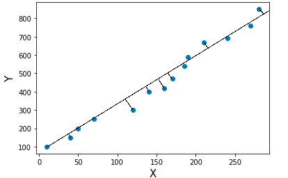
Consider a scatter data and we can fit the data using different straight lines. The line with high variance is called principal component. So using PCA, we get many principal components with different variances. The ordered principal components from high to low are helpful to filter out the low order variance principal component which inturn reduces the data size for model building.
The data analysis is mainly carried out on the features which have more information or high variance.
Variance is a measure of heterogeneity in a dataset. Higher the variance, the data is heterogeneous and smaller the variance, the data is homogeneous.
What is the relationship between eigen values and eigen vectors with principal component?
For the covariance or correlation matrix, the eigen vectors correspond to principal components and the eigen values to the variance explained by the principal components. It is equivalent to fit the straight line with high variance.
So by using the features in a dataset, we can transform the dataset to covariance matrix. By performing Eigen value decomposition or Proper orthogonal decomposition, the eigen values and eigen vectors are decomposed. The eigen vectors are ordered using the magnitude of eigen value which represents the principal components with ordered variance.
Basic mathematical steps to find out principal component
- Standardize the features by transform the data to center it by removing the mean value of each feature, then scale it by dividing non-constant features by their standard deviation.
- Find covariance matrix
- Perform proper orthogonal decomposition to find out eigen values and eigen vectors
- Prioritize the eigen vectors using the magnitude of eigen values from high to low which represents principal components ordered with respect to its variance
Here is a simple example to find out the principal component using the mathematical steps described above.
import numpy as np
import pandas as pd
from sklearn import preprocessing,decomposition
from sklearn import model_selection,metrics
from sklearn.linear_model import LogisticRegression
import matplotlib.pyplot as plt
%matplotlib inline
#Create a DataFrame
data = {
    'Name':['Dinesh','Ramesh','Suresh','Uday','Arun','Madhu','Arjun',
   'Rahul','Rani','Andrew','Ajay','Raj'],
   'Maths':[64,47,56,74,31,77,84,63,42,37,71,59],
   'English':[91,87,67,55,48,72,76,79,45,92,99,69],
   'Biology':[61,86,77,45,73,62,77,89,71,67,96,71],
   'Physics':[89,56,74,41,67,62,99,91,77,71,88,82],
   'Chemistry':[67,87,72,76,73,66,77,55,71,63,99,56]}

df = pd.DataFrame(data)
print(df)
      Name  Maths  English  Biology  Physics  Chemistry
0   Dinesh     64       91       61       89         67
1   Ramesh     47       87       86       56         87
2   Suresh     56       67       77       74         72
3     Uday     74       55       45       41         76
4     Arun     31       48       73       67         73
5    Madhu     77       72       62       62         66
6    Arjun     84       76       77       99         77
7    Rahul     63       79       89       91         55
8     Rani     42       45       71       77         71
9   Andrew     37       92       67       71         63
10    Ajay     71       99       96       88         99
11     Raj     59       69       71       82         56
X = df.iloc[:,1:6]
Standardizing the dataset
X_std = preprocessing.StandardScaler().fit_transform(X)
Transforming the dataset to a covariance matrix
cov_mat = np.cov(X_std.T)
Performing linear transformation to decompose the covariance matrix to eigen values and eigen vectors
eigen_values,eigen_vectors = np.linalg.eig(cov_mat)
print(eigen_values)
[2.1974262 0.22910738 0.61746263 1.18424081 1.22630843]
Eigen vectors are ordered using eigen values to find out the principal components
# Eigenvalue, Eigenvector sorted and reversed from high to low

eigen_pairs = [(np.abs(eigen_values[i]), eigen_vectors[:,i]) for i in range(len(eigen_values))]

eigen_pairs.sort()
eigen_pairs.reverse()

print('Eigenvalues in descending order:')
for i in eigen_pairs:
    print(i[0])
Eigenvalues in descending order:
2.1974262038005423
1.2263084317750919
1.184240809074938
0.617462633536493
0.22910737635839298
total_magnitude = sum(eigen_values)
variance = [(i / total_magnitude)*100 for i in sorted(eigen_values, reverse=True)]
cumulative_variance = np.cumsum(variance)
plt.bar(x=['PC %s' %i for i in range(1,6)],height=variance,width=0.8)
plt.xlabel("Principal Components",fontweight="bold",fontsize = 15)
plt.ylabel("Percentage of Variance",fontweight="bold",fontsize = 15)
plt.title("Principal Component Analysis",fontweight="bold",fontsize = 20)
plt.show()
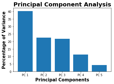
print(variance)
[40.28614706967659, 22.482321249210006, 21.711081499707184, 11.320148281502366, 4.200301899903868]
The first principal component contains 40 % of variance or information about the dataset. So if we consider first 3 principal components, it provides around 83 % of data information.
Here is a example for Classification using Logistic regression with Principal Component Analysis
data = pd.read_table("seeds_dataset.txt", sep = r'\s+', names = 'area,perimeter,compactness,length,width,assymetry,groove_length,variety'.split(","))
The above data and its information below are taken from UCI Machine Learning Repository
(https://archive.ics.uci.edu/ml/datasets/seeds)Data Set Information:
The examined group comprised kernels belonging to three different varieties of wheat: Kama, Rosa and Canadian, 70 elements each, randomly selected for the experiment. High quality visualization of the internal kernel structure was detected using a soft X-ray technique. It is non-destructive and considerably cheaper than other more sophisticated imaging techniques like scanning microscopy or laser technology. The images were recorded on 13x18 cm X-ray KODAK plates. Studies were conducted using combine harvested wheat grain originating from experimental fields, explored at the Institute of Agrophysics of the Polish Academy of Sciences in Lublin.
The data set can be used for the tasks of classification and cluster analysis.
Attribute Information:
To construct the data, seven geometric parameters of wheat kernels were measured:
- area A,
- perimeter P,
- compactness C = 4piA/P^2,
- length of kernel,
- width of kernel,
- asymmetry coefficient
- length of kernel groove. All of these parameters were real-valued continuous.
data.head(5)
| area | perimeter | compactness | length | width | assymetry | groove_length | variety | |
|---|---|---|---|---|---|---|---|---|
| 0 | 15.26 | 14.84 | 0.8710 | 5.763 | 3.312 | 2.221 | 5.220 | 1 |
| 1 | 14.88 | 14.57 | 0.8811 | 5.554 | 3.333 | 1.018 | 4.956 | 1 |
| 2 | 14.29 | 14.09 | 0.9050 | 5.291 | 3.337 | 2.699 | 4.825 | 1 |
| 3 | 13.84 | 13.94 | 0.8955 | 5.324 | 3.379 | 2.259 | 4.805 | 1 |
| 4 | 16.14 | 14.99 | 0.9034 | 5.658 | 3.562 | 1.355 | 5.175 | 1 |
# Check the missing values

print(data.isnull().any(axis=0))
area             False
perimeter        False
compactness      False
length           False
width            False
assymetry        False
groove_length    False
variety          False
dtype: bool
X = data.iloc[:,0:7]
y = data.iloc[:,7]
Feature Standardization
X_transform = preprocessing.StandardScaler().fit_transform(X)
Filtering the principal components which represents about 95 % of variance
# Data with 95% of variance
PCA = decomposition.PCA(0.95)
principal_components = PCA.fit_transform(X_transform)
Thr first 3 principal components reqpresents around 95% of data variance
print(PCA.explained_variance_ratio_)
[0.71874303 0.17108184 0.09685763]
Seed varieties represents “Kama”, “Rosa” and “Canadian”
unique = np.unique(data.variety.values)
print(unique)
[1 2 3]
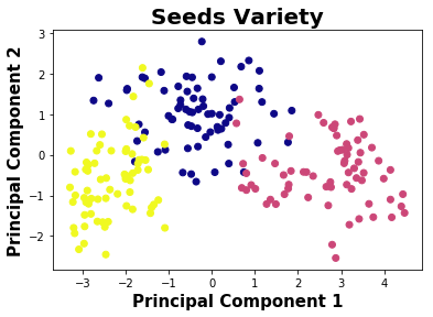
Plotting the seeds variety using first 2 principal components which represents around 89% of the given data
plt.scatter(principal_components[:,0],principal_components[:,1],c=data.variety,cmap="plasma")
plt.xlabel('Principal Component 1',fontweight="bold",fontsize = 15)
plt.ylabel('Principal Component 2',fontweight="bold",fontsize = 15)
plt.title("Seeds Variety",fontweight="bold",fontsize = 20)
plt.show()
# Feature importance using PCA

plt.imshow(PCA.components_.T,cmap ="plasma")
plt.yticks(range(len(X.columns)),X.columns)
plt.colorbar()
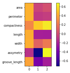
In the above picture, the first 3 principal components contains most of the dataset information.
principal_dataframe = pd.DataFrame(data=principal_components, columns= ["Principal Component 1","Principal Component 2","Principal Component 3"])
target_dataframe = pd.DataFrame({"Target":y})
df = pd.concat([principal_dataframe,target_dataframe], axis = 1)
df.head(5)
| Principal Component 1 | Principal Component 2 | Principal Component 3 | Target | |
|---|---|---|---|---|
| 0 | 0.317047 | 0.783669 | -0.631010 | 1 |
| 1 | -0.003386 | 1.913214 | -0.669754 | 1 |
| 2 | -0.459443 | 1.907225 | 0.932489 | 1 |
| 3 | -0.591936 | 1.931069 | 0.499311 | 1 |
| 4 | 1.102910 | 2.068090 | 0.056705 | 1 |
seed = 1

model = LogisticRegression(penalty='l2',multi_class = 'multinomial',solver = 'newton-cg',random_state = seed)
Model Building using Features
prediction = model_selection.cross_val_predict(model,X_transform,y,cv=10)
matrix = metrics.confusion_matrix(y,prediction)
print(matrix)
[[62  3  5]
 [ 4 66  0]
 [ 4  0 66]]
accuracy = metrics.accuracy_score(y,prediction)
print(accuracy)
0.9238095238095239
report = metrics.classification_report(y,prediction)
print(report)
             precision    recall  f1-score   support

          1       0.89      0.89      0.89        70
          2       0.96      0.94      0.95        70
          3       0.93      0.94      0.94        70

avg / total       0.92      0.92      0.92       210
Model Building using Principal Components
Only considering first 2 principal components which represents around 89% of the given data variance
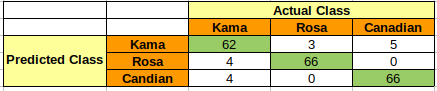
prediction = model_selection.cross_val_predict(model,df.iloc[:,0:2],df.iloc[:,-1],cv=10)
matrix = metrics.confusion_matrix(df.iloc[:,-1],prediction)
print(matrix)
[[60  4  6]
 [ 3 67  0]
 [ 4  0 66]]
accuracy = metrics.accuracy_score(df.iloc[:,-1],prediction)
print(accuracy)
0.919047619047619
report = metrics.classification_report(df.iloc[:,-1],prediction)
print(report)
             precision    recall  f1-score   support

          1       0.90      0.86      0.88        70
          2       0.94      0.96      0.95        70
          3       0.92      0.94      0.93        70

avg / total       0.92      0.92      0.92       210
By comparing the model built using all the features and first two principal components, the accuracy of the model for classification is almost same around 92%.
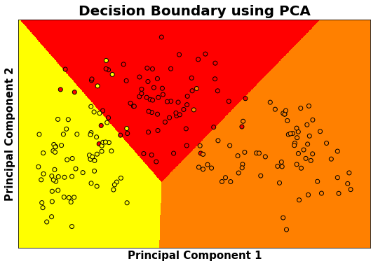
# Decision Boundary using Principal Components

h = 0.01

# Considered the first 2 principal components where around 90 % of variance explained

X = df.iloc[:,0:2]
y = df.iloc[:,-1]

model.fit(X,y)

X_min,X_max = X.iloc[:,0].min()-0.5 , X.iloc[:,0].max()+0.5
y_min,y_max = X.iloc[:,1].min()-0.5 , X.iloc[:,1].max()+0.5

XX,yy = np.meshgrid(np.arange(X_min,X_max,h),np.arange(y_min,y_max,h))

Z = model.predict(np.c_[XX.ravel(),yy.ravel()])

Z = Z.reshape(XX.shape)

plt.figure(1,figsize=(9,6))
plt.pcolormesh(XX,yy,Z,cmap="autumn")

plt.scatter(X.iloc[:,0],X.iloc[:,1],c=y, edgecolors ='k', cmap = "autumn")

plt.xlim(XX.min(),XX.max())
plt.ylim(yy.min(),yy.max())

plt.xlabel('Principal Component 1',fontweight="bold",fontsize = 15)
plt.ylabel('Principal Component 2',fontweight="bold",fontsize = 15)

plt.xticks(())
plt.yticks(())

plt.title("Decision Boundary using PCA",fontweight="bold",fontsize = 20)

plt.show()
References :
- https://scikit-learn.org/
- https://stackoverflow.com/
- https://en.wikipedia.org/
- https://archive.ics.uci.edu/
Comments