
This topic explains the application of Machine Learning using Apache Hadoop and Apache Spark (PySpark MLlib)
What is Apache Spark? Why do we need to use for Big Data Application?
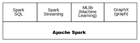
Apache Spark is a unified analytics engine for big data processing, with built-in modules for streaming, SQL, machine learning and graph processing.
The main advantages of using spark for Big Data Applications are
- 100 times faster compared to Hadoop MapReduce computation
- Can be used from Scala, R, Python environment
- It has libraries for processing SQL, Streaming Data, Machine Learning and Graph Computation
- Can be used with Hadoop, Standalone cluster nodes, cloud etc.
How it runs faster than MapReduce?
The Hadoop MapReduce use to read from and write to a disk while Apache Spark speeds up data processing via in-memory computation(RAM)
Here is an example for starting the hadoop in a standalone node and data processing using HDFS
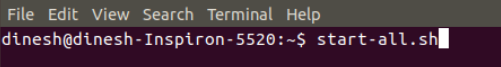
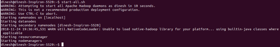
Step 1:
Using the command start-all.sh starts the hadoop daemons all at once
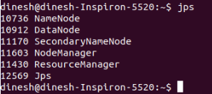
Step 2:
Check the status using command jps in the terminal
Step 3:
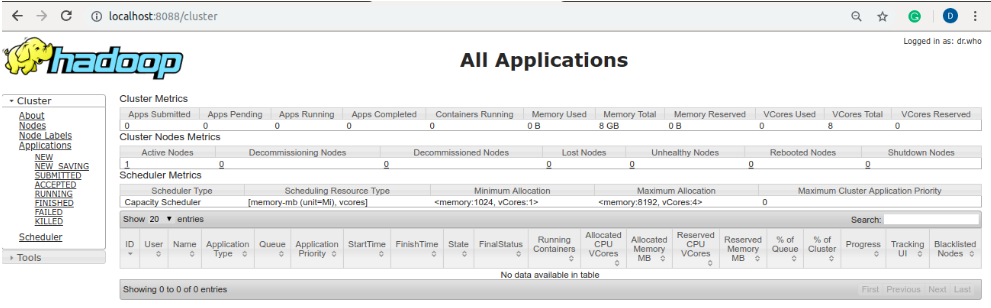
Check the hadoop cluster information and hadoop file system using the browser

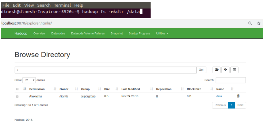
Step 4:
Create a folder in the hadoop root using command hadoop fs -mkdir /folder_name
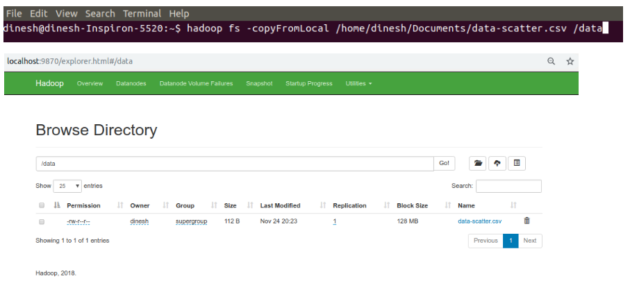
Step 5:
Copy a data file from local to HDFS using below command

hadoop fs -copyFromLocal {Local Path} {Destination Path}
Below program uses the above data from hadoop file system and perform machine learning algorithm using Apache Spark MLlib
from pyspark.sql import SparkSession
from pyspark.ml.feature import VectorAssembler
from pyspark.sql.types import DoubleType
from pyspark.ml.regression import LinearRegression
from pyspark.ml.evaluation import RegressionEvaluator
import matplotlib.pyplot as plt
%matplotlib inline
Spark = SparkSession.builder.appName("ops").getOrCreate()
# Read from Hadoop file system
df = Spark.read.csv('hdfs://localhost:9000/data/data-scatter.csv',header = 'TRUE')
df.show()
+---+---+
|  X|  y|
+---+---+
| 10|100|
| 40|150|
| 50|200|
| 70|250|
|120|300|
|140|400|
|160|420|
|170|470|
|185|540|
|190|590|
|210|670|
|240|690|
|270|760|
|280|850|
+---+---+
df.printSchema()
root
 |-- X: string (nullable = true)
 |-- y: string (nullable = true)
# Converting the string data to double format
df = df.withColumn("X", df["X"].cast(DoubleType()))
df = df.withColumn("y", df["y"].cast(DoubleType()))
df.printSchema()
root
 |-- X: double (nullable = true)
 |-- y: double (nullable = true)
# Transforming the feature and label

data = VectorAssembler(inputCols = ['X'], outputCol = 'feature')
df_tmp = data.transform(df)

#data = VectorAssembler(inputCols = ['y'], outputCol = 'label')
#df_update = data.transform(df_tmp)

df_transformed = df_tmp.select(['feature', 'y'])
df_transformed.show(5)
+-------+-----+
|feature|    y|
+-------+-----+
| [10.0]|100.0|
| [40.0]|150.0|
| [50.0]|200.0|
| [70.0]|250.0|
|[120.0]|300.0|
+-------+-----+
only showing top 5 rows
df_transformed.printSchema()
root
 |-- feature: vector (nullable = true)
 |-- y: double (nullable = true)
# Linear regression using Pyspark
model = LinearRegression(featuresCol = 'feature', labelCol='y', maxIter=10, regParam=0.3, elasticNetParam=0.8)
lr = model.fit(df_transformed)
print("Coefficients: " + str(lr.coefficients))
print("Intercept: " + str(lr.intercept))
Coefficients: [2.730083771254095]
Intercept: 40.09079631232195
ModelSummary = lr.summary
print("RMSE: {},r2: {}".format(ModelSummary.rootMeanSquaredError,ModelSummary.r2))
RMSE: 35.90635015788766,r2: 0.9752919996083498
lr_predict = lr.transform(df_transformed)
lr_predict.select("feature","y","prediction").show(5)
lr_evaluator = RegressionEvaluator(predictionCol="prediction",labelCol="y",metricName="r2")
print("R Squared (r2) for predicted data: {}".format(lr_evaluator.evaluate(lr_predict)))
+-------+-----+------------------+
|feature|    y|        prediction|
+-------+-----+------------------+
| [10.0]|100.0|  67.3916340248629|
| [40.0]|150.0|149.29414716248573|
| [50.0]|200.0|176.59498487502668|
| [70.0]|250.0| 231.1966603001086|
|[120.0]|300.0|367.70084886281336|
+-------+-----+------------------+
only showing top 5 rows

R Squared (r2) for predicted data: 0.9752919996083498
# Converting the Spark DataFrame to Pandas DataFrame
predict = lr_predict.select("prediction").toPandas()
X = df.select("X").toPandas()
y = df.select("y").toPandas()
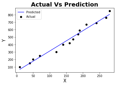
# Plot the Actual data Vs Predicted data
plt.scatter(X,y,color="black",label = 'Actual')
plt.plot(X,predict,color="blue",label = 'Predicted')
plt.xlabel('X', fontsize = 15)
plt.ylabel('Y', fontsize = 15)
plt.title('Actual Vs Prediction',fontweight="bold",fontsize = 20)
plt.legend()
plt.show()
References :
- https://spark.apache.org/
- https://stackoverflow.com/
- https://dzone.com/articles/apache-hadoop-vs-apache-spark
Comments